How Quartet Detects Aircraft from Space
Created by Brady Africk | Updated July 8 2026
Exploiting sub-second timing offsets between Sentinel-2 spectral bands to detect moving aircraft as collinear dot patterns in satellite imagery.
B2 (Blue) · B8 (NIR) · B3 (Green) · B4 (Red)
1 The Key Idea
Sentinel-2 satellites take pictures of Earth using separate color filters — blue, near-infrared (NIR), green, and red — but they don't fire simultaneously. The filters fire in sequence over about one second: NIR ~0.26 s, green ~0.53 s, and red ~1.0 s after blue.
For anything on the ground — buildings, roads, fields — this doesn't matter. They don't move, so they look the same in all four images. But an aircraft moving at 800+ km/h covers about 220 meters in that one-second sequence.
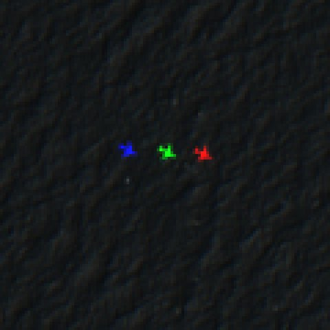
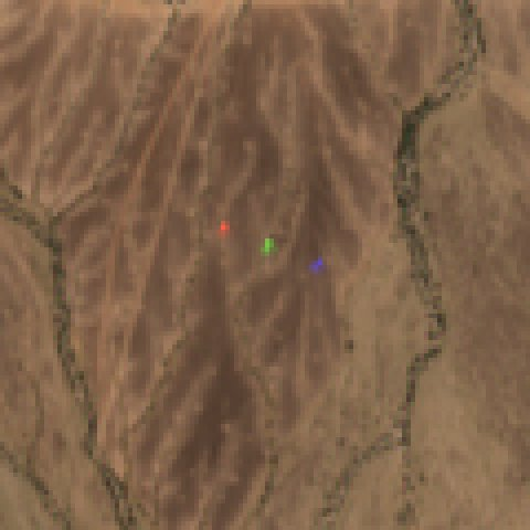
The result: a flying aircraft shows up as four colored dots in a line — blue, NIR, green, red — while everything else on the ground appears as a single, ordinary point.
2 Finding Bright Dots
Aircraft are small (a 737 is about 3-4 pixels wide at this resolution) but surprisingly bright. Sunlight reflects off the metal fuselage, making them stand out against the darker ground below.
Quartet scans each color band separately, comparing every pixel to its local neighborhood. Pixels that are significantly brighter than their surroundings are flagged as candidates. Over a typical satellite tile (~110 km wide), this might find thousands of bright spots per color.
The brightness test also adapts to the scene. It relaxes over dark, calm water so faint over-water aircraft aren't missed, and tightens over clouds, snow, and sun-glint, where natural sparkle can mimic aircraft. (The detailed view explains the mechanics.)
3 Matching Triplets
Most bright spots are just noise — rooftops, wave crests, mineral deposits. Quartet filters them by looking for the specific pattern that only a moving aircraft produces: three dots in a straight line with the right spacing (the blue, green, and red dots — the fourth, NIR dot joins in step 5).
The spacing between dots depends on the aircraft's speed (faster = wider spacing), and the line direction reveals its heading. The green-red gap is roughly 0.907× the blue-green gap (set by the satellite's band-capture timing — 0.478 s vs 0.527 s), which provides a strong geometric test.
Of thousands of bright spots, typically only a handful form valid triplets.
4 AI Scoring
Even after geometric filtering, some false matches slip through — cloud edges, contrails, or coincidental alignments of bright features. Quartet uses a machine learning model (XGBoost) trained on ~43,000 human-labeled examples to score each candidate.
The model examines 53 characteristics of each candidate: Is the dot bright in its own band but not in the other bands? (Aircraft dots only appear in one band at each position.) Is there a contrail trailing behind? How uniform is the surrounding terrain? Is the speed physically plausible? Does the parallax-corrected speed look like a real cruise value? Is the sun positioned to cause sun-glint on water? Is the atmosphere hazy or dusty in a way that would weaken normal aircraft signatures?
Candidates scoring above 60% confidence are kept as detections. The model's holdout F1 score is 0.979 (high precision and high recall — very few false alarms, catches almost every aircraft).
5 The Fourth Band: Near-Infrared
Sentinel-2 also captures a near-infrared (NIR) band, invisible to human eyes but captured between the blue and green bands. This gives Quartet a fourth dot for each aircraft.
Four dots are better than three: the extra point confirms the detection is real (noise rarely produces four collinear dots at the right relative spacing) and improves speed/heading accuracy.
6 Verification with Flight Data
If you flip the ADS-B On toggle for a search, Quartet cross-references detections with ADS-B flight tracking data — the same data used by sites like FlightRadar24. If a detection matches a known aircraft's position and timing, Quartet shows the aircraft's registration, callsign, altitude, and type.
This verification step confirms the detection is real and adds context. Unmatched detections may be military aircraft, private flights without ADS-B transponders, or (rarely) false positives.
7 Imagery from Multiple Providers
Satellite imagery for any given date comes from multiple providers — Element84, Microsoft Planetary Computer, and CDSE. If one provider is lagging or missing a specific tile, Quartet automatically falls through to the next. You never have to think about where the data is coming from; the search just works. Tile imagery is cached on the server so repeat views are instant.
Real Examples from Sentinel-2
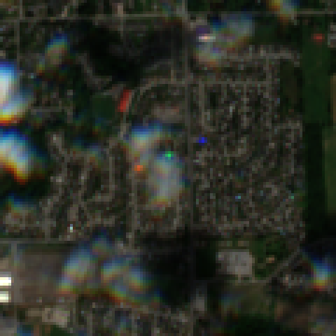
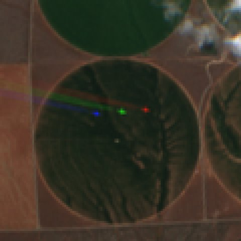
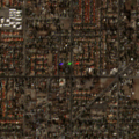
Each image below shows an actual aircraft detected in satellite imagery. Look for the blue, green, and red dots separated along the flight path.
By the Numbers
Switch to Detailed view for the full technical deep-dive.
The Core Principle
Most satellite imagery captures each spectral band at a slightly different time. Quartet turns this apparent limitation into a detection mechanism.
The Copernicus Sentinel-2 constellation (S2A, S2B, S2C) carries identical Multi-Spectral Instruments (MSI) with push-broom sensors. Unlike a camera that captures all colors simultaneously, the MSI records each spectral band through a separate detector array, offset along the satellite's flight direction.
For stationary objects, this timing difference is invisible. But a moving aircraft travels a measurable distance between band captures, appearing at a different pixel position in each band.
In an RGB composite, this produces a distinctive triplet pattern — three separated colored dots (blue, green, red) arranged along the flight path. The near-infrared (B8) band adds a fourth confirmation dot, strengthening the geometric constraint.
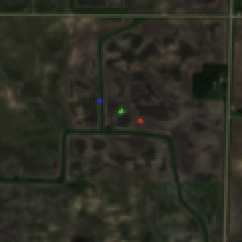
Each image below shows an aircraft detected in Sentinel-2 imagery. The colored dots — blue, green, and red — appear separated along the flight path because the satellite captures the bands in sequence: green ~0.53 s after blue, red ~1.0 s after blue. The background varies from open ocean to farmland, but the triplet signature is unmistakable.
Push-Broom Scanning & Band Timing
Four spectral bands are captured with precise, known time delays — forming the geometric basis for detection and the collinearity constraint.
The 0.907 Ratio
The time gap between green and red (0.478s) divided by the gap between blue and green (0.527s)
gives a constant ratio of 0.907. For an aircraft flying straight at constant speed,
the green-to-red pixel displacement is exactly 0.907× the blue-to-green displacement.
This ratio acts as a powerful geometric fingerprint — random bright pixel alignments
almost never satisfy this constraint.
NIR Extends the Constraint
The B8 (NIR) band sits between B2 and B3 on the focal plane, adding a fourth collinearity point. Its position relative to the RGB triplet depends on detector parity:
- Odd detectors: scan B2→B8→B3→B4 — NIR at
0.501×blue→green - Even detectors: scan B4→B3→B8→B2 (reversed) — NIR at
0.501×green→blue
The detector parity is determined from the ESA granule_metadata.xml viewing angle grids for each tile.
With four time points, the velocity regression becomes overdetermined — three collinear points always
fit a perfect line, but a fourth point reveals real deviations, making scatter_m a genuine
goodness-of-fit metric. The separate scatter_3band_m feature captures the RGB-only residual,
so the model can measure how much the NIR point improved (or worsened) the fit.
The Detection Pipeline
Each Sentinel-2 tile flows through six sub-steps that progressively narrow thousands of bright pixel candidates down to verified aircraft detections.
3.1 Bright Pixel Extraction
Aircraft fuselages are metallic and highly reflective. For each band independently:
- Estimate local background using a uniform (mean) filter
- Compute residuals (original − background)
- Estimate noise via Median Absolute Deviation (MAD)
- Flag pixels exceeding background by both 3.5σ and an adaptive floor that scales with local noise — then apply per-pixel scene-aware overrides for cloud, snow, and sun-glint conditions
σ = max(1.4826 × MAD, 0.002)
// Adaptive floor: looser over very dark water,
// reverts to the constant 0.025 cap elsewhere
floor = max(0.0175, min(0.025, 5 × σ))
// Per-pixel overrides via Scene Classification Layer (SCL):
// cloud / snow / cirrus pixels stay pinned at static 0.025
if SCL in {8, 9, 10, 11}: floor = 0.025 // CLOUD_MED, CLOUD_HIGH, CIRRUS, SNOW
// Scene-level glint guard: when sun-glint geometry is bad,
// EVERY pixel gets the strict floor regardless of SCL class
if glint_angle < 20°: floor = 0.025 // global guard
// Threshold for "bright" classification
threshold = max(3.5 × σ, floor)
- Adaptive floor for dark water: Over very dark water, the local noise floor σ is so small that aircraft dots can fail a flat 0.025-reflectance threshold — the absolute excess is just too low. Scaling the floor with σ (5σ below the cap, capped at 0.025 above) recovers these faint over-water aircraft while preserving baseline behavior wherever the local noise is meaningful.
- 0.9 reflectance ceiling: Pixels above 0.9 reflectance are excluded from the bright-pixel pool entirely — saturated specular reflections (ice, sun-glint blowout, polished metal roofs) where the band-by-band dot pattern is destroyed by clipping. Aircraft dots at typical altitudes don't approach 0.9, so the ceiling cleanly removes the noisy long tail without TP loss.
- Per-pixel SCL overrides for clouds, snow, and cirrus: Cumulus cloud edges, snow, and cirrus pixels produce dense fields of bright candidates that look indistinguishable from aircraft dots to the geometric matcher — bloating the candidate pool 100× on dense scenes without producing real detections. Pinning these pixels to the static 0.025 floor filters the noise without excluding real aircraft. Cirrus is included in this set; on dense cirrus tiles the matcher's rescan cap saturates without the override. The cirrus FP/TP penalty (training-data ratio 0.76) is accepted for the recall recovery.
- Global glint guard for bad sun-glint geometry:
When sun-glint geometry is bad (
glint_angle< 20°, computed from the full sun-vs-sensor specular geometry — not just view angle), the entire scene is at high FP risk: wave glint over water, cirrus glint, and bright sand/soil specular reflections all spike together. Filtering just the worst SCL classes left enough noise in the others to saturate the rescan cap. The global guard elevates every pixel in the scene to the strict floor under bad-glint geometry. Benign-glint scenes (~90% of the world) see zero behavior change.
3.2 Clustering
Adjacent bright pixels are grouped via connected-component labeling:
- 1–35 px: Kept as candidates (centroid becomes detection point)
- 36–50,000 px: Split using DBSCAN to recover sub-clusters (e.g. aircraft dot embedded in a contrail)
- >50,000 px: Rejected (pathologically large blobs)
3.3 Triplet Matching
The core detection step uses vectorized batched KD-tree queries and direct C-level data structures to match all candidates simultaneously, eliminating per-candidate Python loops at every stage:
- Batch B→G query (sparse_distance_matrix):
A single
cKDTree.sparse_distance_matrix(other, r, output_type='ndarray')call finds all blue–green pairs and returns a flat numpy record array with(i, j, distance)fields directly from C — no Python list-of-lists intermediate, and the distance is precomputed (no downstreamnp.hypotcall needed). - Vectorized B-G filtering: Numpy array ops compute all displacement vectors and discard sub-minimum separations in one mask operation
- Batch red prediction: All predicted red positions are computed at once, then a single batched
query_ball_pointwith per-pair variable radii finds red candidates - Two-pass G-R flatten: The variable-radii GR query
doesn't fit
sparse_distance_matrix, but the same Python-list overhead is skipped via a two-pass allocate-then-fill pattern: count total pairs, allocate exact-size numpy arrays, fill via slice-assignment from the C-returned neighbor lists. Bit-identical output to list-extend; 20–50% faster. - Vectorized validation: Collinearity (≤20°), spacing ratio (0.907 ± 0.3), and distance checks are applied as parallel numpy boolean masks
- Vectorized survivor processing:
Parallax correction and speed computation are batched across all surviving triplets
via
_correct_parallax_batchand_compute_parities_batchhelpers (one numpy call covers all M survivors instead of M scalar function calls). ~10× faster on dense scenes; output bit-identical to per-survivor scalar loop. - Lazy gather of position arrays:
Only the 4 arrays validation needs (
t_bg_vecs,t_bg_dists,t_g_pos,t_r_pos) are gathered eagerly. The other 3 (t_bi,t_gi,t_b_pos) are deferred until after the survivors mask, and validation intermediates (gr_vecs,dot_products,cos_angles) are explicitly freed between steps.
redpredicted = green + (green − blue) × 0.907
// Validation constraints (applied as numpy boolean masks)
collinearity: angle(BG, GR) ≤ 20°
spacing ratio: |dGR/dBG − 0.907| ≤ 0.3
Greedy best-first assignment ensures each bright pixel cluster is used in at most one triplet, sorted by geometric quality.
3.4 Residual Re-Scan
After greedy dedup, the matched clusters are removed from each band's candidate list and matching runs again on the residual centroids. This catches aircraft "shadowed" by nearby detections in the first pass — e.g., close-formation pairs where one aircraft's green cluster was closer to the other's blue.
A second residual pass runs after ML scoring (step 3.6, below): when a junk triplet with good geometry steals a real aircraft's dot during dedup, then gets rejected by ML, the dot is freed. The algorithm looks back at all raw (pre-dedup) triplets whose dots are now unclaimed and scores them through the full ML pipeline to recover the missed aircraft.
On dense scenes (cities, sun glint, partial cloud cover) the residual pool can balloon
into the hundreds of thousands or even millions of triplets. To bound worst-case latency
without measurable recall loss, the residual list is capped at
100,000 triplets, sorted by the same
geometric cost metric the greedy dedup uses (|ratio − 0.907| + angle/180).
Triplets with the cleanest collinearity and ratio rank to the top and are kept; the noisy
long tail is discarded.
Geometry-cost ranking alone can still drop a genuine aircraft in extremely dense sub-tiles, where the real triplet ranks worse on collinearity/ratio than thousands of competing candidates. To cover this, a second, additive rescan track ranks the same candidate pool by brightness (minimum cross-band excess) and unions up to 50,000 brightness-selected triplets into the geometry track. Because it only ever adds candidates, it can never discard a geometry survivor. Detections recovered solely by the brightness track are tagged so heavy-glint scenes can be mined as hard negatives — bright glint triplets the current model still scores highly.
The 100K value bounds rescan latency without measurable recall loss: real-TP geometric cost on dense cirrus tiles can rank anywhere in the top 100K. The cap is paired with the cirrus + global-glint floor widening (which trims input candidate counts by 3-5× on dense sub-tiles) so the 100K cap mostly catches what's left rather than driving major work itself. The pool is built incrementally via a streaming chunk consumer + bounded heap to avoid materializing the full residual list in memory.
3.5 Velocity & Heading Computation
With three positions and three known timestamps, ground speed and heading are computed via closed-form 2D linear regression:
// 3-band (RGB only) — indices align with [B2, B3, B4] position arrays
t = [0.000, 0.527, 1.005] seconds
// 4-band (RGB + NIR) — indices align with [B2, B3, B4, B8] position arrays
// (NIR appended last by index, but captured between B2 and B3 in time)
t = [0.000, 0.527, 1.005, 0.264] seconds
// Closed-form OLS velocity
vrow = Σ((t − t_mean) × positions) / t_ss
speed = √(vrow² + vcol²) × pixel_size × 3.6 → km/h
With 3 bands, scatter is always near-zero (3 points define a line). With 4 bands (NIR), scatter becomes a genuine goodness-of-fit metric — real aircraft produce scatter under 10m; false alignments don't survive the 4th point.
3.6 ML Confidence Scoring
Each candidate is scored by an XGBoost classifier trained on ~43,000 user-labeled examples (F1 = 0.979, AUC = 0.996). The model outputs a probability (0–100%) and candidates below 60% are discarded. The model uses 53 features across ten categories (see ML section below).
Several FP-relevant signals are exposed as ML features rather than hard gates —
spectral_ratio (cross-band variance) is one example. Aircraft tend to have low
cross-band variance, but the model decides the threshold rather than a fixed cutoff. The
bulk of FP rejection (rooftops, cloud edges, glint, ship wakes) happens here, in the
classifier — learned features discriminate these classes more accurately than fixed
thresholds.
ML Feature Architecture
The XGBoost model evaluates candidates across 53 engineered features spanning geometry, spectral properties, spatial context, cross-band isolation, contrail detection, NIR confirmation, altitude-sensitive parallax discrimination, derived cross-feature ratios, sun-glint geometry, and atmospheric conditions (aerosol optical thickness and water vapor).
Bar length = XGBoost per-split gain importance (retrain #58, May 2026), one scale across all groups; features below the scale floor render at minimum width. Multi-feature rows (e.g. per-band peaks) show the mean of their per-band gains.
Cross-Band Isolation
A key discriminator: at each band's detection position, the correct band should be significantly brighter than the other bands (because the aircraft has moved). Static objects appear equally bright in all bands at the same position. The cross-band excess features are the model's most important signal by gain.
Under thin cirrus or haze, all bands become equally bright due to the atmospheric veil,
pushing cross_band_excess toward zero even for real aircraft. The
floor-subtracted variants (cross_band_floor_excess) address this
by subtracting the median excess across all three bands at each position — removing the
correlated atmospheric component while preserving the aircraft's band-specific signal. In the
current model, the floor-subtracted variant min_cross_band_floor_excess is in
fact the single highest-gain feature of all 53.
Atmospheric Context (AOT & WVP)
Two features sampled from the Sen2Cor L2A atmospheric correction products tell
the model when to trust the parallax cascade and when the imagery itself is degraded:
aot_value (Aerosol Optical Thickness, τ) flags hazy or cirrus-affected
scenes, and wvp_value (Water Vapor, g/cm²) carries complementary
information about humid atmospheres.
High-confidence FPs over arid land or cirrus and missed-aircraft tails over humid atmospheres tend to have elevated AOT (τ ≈ 0.15–0.18) versus clean baselines (τ ≈ 0.10). The features act bidirectionally: the model uses them as an ‘atmospheric quality’ calibration channel rather than a global reject signal — high atmosphere readings tell XGBoost to weight the cross-band cascade less harshly when other features still support an aircraft, and to lean FP when cross-band is also weak.
AOT is preferred over the B10 (1.375 µm cirrus band) signal because Sen2Cor already uses B10 internally and combines it with surface-model context for a regional atmospheric estimate — AOT carries that combined information. B10 also requires a separate L1C STAC, a different S3 bucket (requester-pays), and JP2 instead of COG.
Contrail Detection
The algorithm scans bidirectionally along the heading for a bright trail in the combined RGB mean, up to 50 pixels (~500m) in each direction. Contrails appear in all bands simultaneously (unlike the triplet dots) and trail behind the aircraft. A perpendicular width check distinguishes real contrails (1–2 px) from landscape features like field edges and cloud boundaries (wider). If width exceeds 2 px, all contrail features are zeroed out to prevent the model from learning false contrail signals. When a valid contrail is detected, a pixel-level contrail mask is built and nearby features are recomputed to avoid contamination.
Two-Pass Optimization
Contrail analysis is expensive (pixel-level scanning per detection). When more than 500 triplets are found, the pipeline uses a two-pass approach: first extract fast features (skipping contrail analysis) and ML-score all candidates at a relaxed threshold (half the normal threshold, i.e., 30% instead of 60%). This allows aircraft that need contrail features to boost their score to survive the pre-filter. Only survivors then get full contrail analysis in pass two, and are re-scored at the normal 60% threshold.
Sun-Glint Geometry
Over open water, the dominant false-positive class is sun glint — sparkle fields on wavelets that produce triplets of bright sub-pixel peaks coincidentally arranged along the aircraft time axis. The spatial features alone (brightness, collinearity, cross-band isolation) can be fooled because each wavelet peak is a compact bright broadband source, identical in character to an aircraft dot.
What these FPs share is geometry: the sensor happens to be looking near the specular reflection direction of the sun off a flat water surface. The detector computes three geometric features for every scene (view angles + sun position + tile center; no imagery needed), applied identically to every detection in a tile:
glint_angle— the angle between the sensor's view direction and the specular direction (sun mirrored across local vertical). 0° = staring at the bright spot; 45°+ = safe.sun_elevation— degrees above horizon at the sensing time. Higher sun means stronger direct illumination.rel_azimuth— azimuthal offset between view and specular direction, wrapped to [0, 180°]. Complementsglint_anglewhen elevation alone is weak.
Over-water univariate discrimination (AUC) on the training set is 0.82 — comparable to the cross-band parallax features. Over land the signal correctly drops to noise level (AUC ≈ 0.51), and the model learns to ignore it there. Sensing time for the computation is resolved via a four-tier chain (explicit STAC timestamp → full tile ID → short tile ID date + ~10:30 mean-local-solar-time approximation → neutral defaults), so every row gets a value even if one source is missing.
Derived Cross-Feature Ratios
Seven additional features are computed from existing measurements, requiring no extra data downloads:
| Feature | Formula | Why It Matters |
|---|---|---|
| nir_spectral_ratio | nir_peak / mean_brightness | Aircraft reflect roughly equally across NIR and visible bands (ratio ≈ 1.0); vegetation is much brighter in NIR, water much dimmer |
| ndvi | (nir_peak − peak_red) / (nir_peak + peak_red) | Vegetation has high NDVI; metal aircraft have low or negative NDVI |
| velocity_uncertainty | scatter_m / pixel_separation | Normalized fit quality — low for fast, well-separated real aircraft |
| excess_consistency | std(excess_B, excess_G, excess_R) / mean_excess | Real aircraft have consistent excess across bands; artifacts are uneven |
| spectral_ratio_4band | max(peak_B, peak_G, peak_R, nir_peak) / min(…) | 4-band version — NIR adds a constraint; FPs tend to have one anomalous band |
| excess_consistency_4band | std(excess_B, excess_G, excess_R, nir_excess) / mean | 4-band uniformity check — stronger separation than the 3-band variant |
| speed_per_sep | speed_kmh / pixel_separation_px | Parallax-quality ratio — false positives cluster at a characteristic value, real aircraft scatter with altitude-correction quality |
NIR Band (B8) — The Fourth Dimension
Adding the near-infrared band transforms the three-point triplet into a four-point collinearity test, dramatically reducing false positives.
Sentinel-2's B8 (NIR) band is captured at 10-meter resolution — the same native resolution as the visible RGB bands. On the MSI focal plane, B8 sits between B2 (Blue) and B3 (Green), captured 0.264 seconds after B2. This means the NIR dot appears roughly halfway between the blue and green dots, not beyond red as one might expect from the band numbering.
How NIR Detection Works
- Predict NIR position from the blue→green displacement vector:
nir_pred = blue + (green - blue) × 0.501(odd detectors; even detectors anchor on green with the same 0.501 fraction, reflecting the reversed focal-plane order) - Search 15×15 window (±7px) around prediction for the actual NIR peak; the match is only accepted if the found peak lies within 6 px of the predicted position
- Compute collinearity: Euclidean distance from predicted to actual peak
- Compute NIR excess: Peak brightness minus local background
- Cross-band check: At the NIR position, NIR excess should exceed B/G/R excess
The Five NIR Features
| Feature | What It Measures | Why It Matters |
|---|---|---|
| nir_excess | NIR 3×3 peak minus background | High for real aircraft (metallic NIR reflectance) |
| nir_peak | Raw NIR reflectance at peak | Aircraft fuselages are bright in NIR |
| nir_cross_excess | NIR excess minus max(B/G/R excess) at same position | True 4-band cross-check — aircraft has moved since RGB capture |
| nir_collinearity | Distance from predicted to actual NIR peak (pixels) | Low for real aircraft; the NIR match is accepted up to 6px from prediction. High for false positives |
| nir_distance_ratio | dist(blue, NIR) / dist(blue, green) | Real aircraft ≈ 0.50 (B8 halfway between B2 and B3); FPs often exceed 1.0 |
4-Band Velocity Fit
With B08 as a fourth data point, velocity is computed via ordinary least-squares regression
across all four band positions instead of the three-point fit used with RGB alone. Three
collinear points always fit a line perfectly, so the scatter_m residual is always
zero. With four points, scatter becomes a genuine goodness-of-fit metric — real aircraft
produce low scatter (<10 m), while coincidental three-point alignments that fail the
fourth-point test produce large residuals.
The model also receives scatter_3band_m — the RGB-only residual evaluated
against the 4-band velocity fit. If a spurious NIR "dot" pulls the fit away from the
true RGB line, scatter_3band_m rises while scatter_m stays low,
exposing the false NIR match. For real aircraft, both values are similar.
nir_collinearity=99, others -1)
that the model can distinguish from real measurements. The 4-band derived features
(spectral_ratio_4band, excess_consistency_4band) also revert to
sentinels rather than silently falling back to their 3-band equivalents — this lets the
model learn separate decision boundaries for 3-band and 4-band cases. Velocity falls back to
the 3-band fit, and the model relies on the remaining 44 non-NIR features (the NIR-derived
ratios nir_spectral_ratio and ndvi revert to sentinels too).
ADS-B Cross-Validation
Detected aircraft are cross-referenced against ADS-B transponder data to identify which real-world aircraft each detection corresponds to.
ADS-B (Automatic Dependent Surveillance-Broadcast)
is a system where aircraft continuously broadcast their position, altitude, speed, and identification.
Quartet merges up to three ADS-B sources into a single aircraft index — two daily archives,
ADS-B Exchange globe_history
and adsb.lol (2023+), plus
Flightradar24
live playback for the last 7 days. The archives are keyed by ICAO hex, so overlapping
aircraft collapse cleanly; FR24's bbox feed uses synthetic flight IDs, so it is deduped against
the hex-keyed sources in three tiers — callsign, then registration, then type + trajectory
(same aircraft type, altitude within ±10 m, heading within ±2°, position within
2.5 km at the same epoch) — and only contributes aircraft the archives missed.
Each detection's apparent coordinates (uncorrected image position) are used for matching — not the parallax-corrected positions. ADS-B positions are real GPS coordinates, so they must be compared to where the aircraft visually appears in the image after the satellite’s off-nadir viewing displaces it.
ADS-B positions are re-interpolated from raw trace data to each detection's exact sensing epoch (accounting for push-broom row timing), rather than using a single tile-center timestamp.
To guard against sparse or noisy trace data (especially FR24), a re-interpolated position that would imply a physically-impossible jump from the tile-center estimate is rejected, falling back to the trusted tile-center interpolation — so a single trace outlier can't push a real match outside the radius. Non-finite (NaN/inf) interpolations are always discarded.
When multiple ADS-B aircraft fall within the match radius of multiple detections, the pairing is resolved by a globally optimal one-to-one assignment — see the Confidence-Weighted Matching section below for the cost function and algorithm.
Aircraft present in ADS-B but undetected are reported as “missed,” but only after a swath filter: an aircraft whose position at sensing time falls in a gap between irregular tile footprints — or in a tile missing on that date — was never in any imagery, so it is excluded rather than counted as a missed detection. This keeps the false-negative count honest when the requested area extends past the tiles actually returned.
Orbit Timing & Parallax
Precise ADS-B matching requires computing the exact moment each pixel row was scanned and correcting for off-nadir viewing geometry.
Sentinel-2 orbits at ~786 km altitude in a sun-synchronous orbit at ~7.44 km/s orbital velocity (~7.0 km/s ground track), scanning north-to-south in ~290 km wide strips.
Per-Tile Sensing Times
Element84 Earth Search provides accurate per-tile sensing times with sub-second precision. CDSE returns only the datatake start timestamp (same for all tiles), which can be 6+ minutes too early.
Tile A: 16:43:18.209 (38.3°N — scanned first)
Tile B: 16:43:32.590 (37.4°N — scanned 14.4s later)
// CDSE gives only the datatake start for both:
Both: 16:37:11.024 (6+ minutes too early!)
Along-Track Parallax Correction
The satellite moves north-to-south at ~7.0 km/s ground track speed while scanning. An aircraft at altitude h appears shifted toward the satellite (northward) by a fraction proportional to its altitude. Each band is captured at a different time, so the parallax shift differs per band — distorting the apparent triplet geometry.
parallax_frac = altitude / 786,000 m
// e.g. 10,000 m / 786,000 m ≈ 0.01272 (1.27% of satellite displacement)
// Correction per band: add parallax_frac × satellite_displacement to row positions
// This undoes the northward apparent shift
rowcorrected = row + parallax_frac × (sat_speed × Δt / pixel_size)
The initial detection (Phase 1) assumes 10,000 m altitude. After ADS-B
matching reveals the true altitude, a Phase 2 pass overwrites heading, speed,
and altitude with the ADS-B values, then re-runs the parallax correction with the
actual altitude (both along-track via recompute_heading_with_altitude
and cross-track via the formula below). This also fixes the 180° heading
ambiguity for northbound aircraft (see callout below) by trusting the ADS-B
heading-of-record over the geometry-derived value.
Detections without an ADS-B match never receive Phase 2, so their reported speed, heading, and pixel separation stay computed at the assumed 10 km altitude. Low, slow aircraft are over-corrected and read too fast — a ~230 km/h light aircraft can appear as ~500 km/h — so the UI flags these values as altitude-assumed rather than measured.
Cross-Track Parallax Correction
Separately, the off-nadir viewing angle creates a cross-track displacement. Aircraft away from the satellite's ground track appear shifted outward from their true position. After ADS-B matching provides the true altitude, this is corrected:
Δd = altitude × tan(incidence_angle)
// Re-correction after ADS-B match (actual vs assumed altitude)
Δ_altitude = actual_alt − 10,000 m
Δ_displacement = Δ_altitude × tan(incidence_angle)
lon += Δx / (111,000 × cos(lat))
lat += Δy / 111,000
View-Geometry Priority
The cross-track formula needs a per-detection viewing angle. Three priority tiers, in order:
- Per-detector grid from
MTD_TL.xml(preferred). The tile's 23×23 view-zenith and view-azimuth grids are fetched alongside the detector parity map;get_view_geometry_at_pixel(blue_pos[0], blue_pos[1], det_map, view_angle_map)looks up the angle for the specific detector covering each detection's pixel. - STAC scene-mean (last-resort fallback). Used when the per-detector
lookup returns
(None, None)— e.g. the granule_metadata.xml fetch failed or the cell is no-data. Can be ~180° wrong on tiles straddling the satellite ground track: the scene-mean averages viewing angles across both swath halves and aliases the bimodal distribution to a meaningless midpoint, which is why the per-detector grid is preferred whenever it's available. - Skip parallax (last resort). When neither tier yields a finite angle pair, the shift is omitted entirely. Distance accuracy degrades by ~h·tan(view_inc) (~1 km at 10 km altitude), but the matching radius absorbs most of that.
Altitude-Sensitive ML Features
The parallax correction creates a powerful discriminator: compute the apparent speed twice — once assuming ground level (h=0) and once with the default correction (h=10 km). The difference reveals whether the object is airborne.
| Feature | What It Measures | Why It Matters |
|---|---|---|
| speed_at_ground_kmh | Apparent speed with zero parallax correction | Ground FPs show extreme values (median 1240 km/h); real aircraft are moderate (median 738 km/h) |
| speed_delta_kmh | Difference between ground and corrected speed | Large delta = object is at altitude; near-zero = ground level |
| heading_delta_deg | Heading change between ground and corrected | Parallax correction changes heading more for along-track aircraft |
| along_track_fraction | Fraction of motion along satellite track | Along-track aircraft are most affected by parallax; cross-track are least |
Confidence-Weighted Matching
The matching algorithm pairs each satellite detection with the most likely ADS-B aircraft, using detection confidence as the primary criterion rather than distance alone.
Match Radius: 2,500 m base, adaptive to 7,500 m
| Error Source | Raw | After Correction | Notes |
|---|---|---|---|
| ADS-B temporal granularity | ~1,250 m | ~200 m | ~5 s snapshot intervals (≈1,250 m at 900 km/h); interpolation to the sensing epoch removes most of it — the residual is the “interpolation error” row |
| Tile sensing time | up to ~30,000 m | ~0 m | Linear orbit-anchor formula error grows toward swath ends — up to ~120 s for tiles 55° south of an 80°N max-north datatake (~30 km at 900 km/h). Fixed by fetching per-tile SENSING_TIME from MTD_TL.xml on MPC, with CDSE S3 fallback for fresh scenes. |
| Cross-track parallax | ~1,000 m | ~50 m | Re-corrected using ADS-B altitude |
| Green band offset | ~130 m | ~0 m | Detection references green (t+0.527s) |
| Interpolation error | ~200 m | ~200 m | Linear interpolation during turns |
| Per-pixel incidence | 100–800 m | 100–800 m | Tile-mean used as approximation |
Scoring Formula
R = min(2500 + ages × 150, 7500)
// Speed nudge: fractional detection-vs-ADS-B speed mismatch,
// scaled to the radius
speed_penalty = |Δspeed| / speedadsb × 0.10 × R
// Combined score (lower = better match)
// Heading penalty is disabled (weight = 0) because apparent
// 180° flips in band-derived heading made it unreliable.
score = (1.0 − confidence) × R + distancem × 0.3 + speed_penalty × 0.10
The radius grows by 150 m per second of ADS-B data age (time since the aircraft
was last seen in a snapshot), capped at 7.5 km. This accounts for the increasing positional
uncertainty when extrapolating stale ADS-B positions.
(1−0.99)×2500 + 2400×0.3 = 25 + 720 = 745.
A 75% confidence detection at 500m scores
(1−0.75)×2500 + 500×0.3 = 625 + 150 = 775.
The high-confidence detection wins despite being farther away.
Optimal Assignment
When multiple aircraft compete for the same detection, a cost matrix is built and solved
using the Hungarian algorithm
(scipy.optimize.linear_sum_assignment) for globally optimal 1:1 matching.
Data Sources & Aircraft Signatures
All imagery comes from the ESA Copernicus program. Detection runs entirely on Quartet's own pipeline — no third-party detection or ML services are involved.
| Component | Source | Details |
|---|---|---|
| Scene Discovery | CDSE STAC + Element84 STAC | Queried together at scene-aggregation; E84 supplies per-tile sensing datetimes where it has them, CDSE covers the remainder. Antimeridian-crossing AOIs are split into two queries. |
| Band Download | 4-tier fallback: E84 → MPC → CDSE S3 direct → CDSE STAC+S3 | Element84 COGs (fastest, public S3), Microsoft Planetary Computer COGs (SAS-signed, fills E84 ingest gaps, ~40% of S2B tiles on some dates), CDSE S3 direct (uses pre-resolved s3:// URLs from STAC merge), CDSE STAC+S3 (re-discovers via CDSE STAC then reads JP2 — catches fresh acquisitions like same-day S2C before they propagate to E84/MPC; the authoritative final tier). When all four miss, the tile reports “imagery not available.” Per-provider 429 cooldown + Retry-After respected. |
| Band Imagery | Cloud-Optimized GeoTIFFs | B02, B03, B04, B08 at 10m; SCL at 20m (upsampled); AOT and WVP atmosphere products at 60m (feed the two atmospheric ML features). E84 entries missing NIR or SCL automatically route to MPC where the full band set is available. |
| Per-Tile Sensing Time | 4-tier cascade: MTD_TL.xml → E84 anchor lerp → max_north derivation → leave alone | Step 0: MTD_TL.xml's microsecond-precision SENSING_TIME fetched via an 8 KB range request on MPC's granule-metadata asset, with a CDSE S3 fallback for fresh scenes still inside MPC's ~24h ingest window (notably S2C). Cached 24h per tile_id. Step 1: for any datatake-start scene that MTD_TL missed, interpolate from the nearest E84 per-tile anchor in the same orbit (lat-difference × 111 km / 7 km/s). Step 2: if neither MTD_TL nor an E84 anchor is available, fall back to datatake-start + _get_orbit_max_north derivation (errors O(60-150 s)). Step 3: leave datetime untouched if all three tiers fail — downstream degrades gracefully. The cascade exists because lat-velocity isn't constant in a sun-synchronous polar orbit, so a single linear orbit-anchor formula has up to ~120 s error on tiles imaged 55° south of the datatake's max-north anchor. |
| ADS-B Data | ADSBx globe_history + adsb.lol (merged by default) + FR24 (auto, last 7 days) | Source mix is gated by the ADSB_SOURCE env var. The default (both) merges ADSBx globe_history and adsb.lol (daily archive, 2023+) by ICAO hex; adsbx or adsblol restrict to a single archive. FR24 (live playback, last 7 days) is consulted unconditionally for dates inside its window and merged via callsign, registration, then type + trajectory, since its bbox feed uses synthetic flight IDs. Positions are ~5 s snapshots (ADSBx); per-aircraft traces report every ~5–30 s, FR24 sparser. |
| ML Model | XGBoost (in-pipeline) | 53-feature classifier, periodically retrained from reviewed user feedback — runs inside Quartet, not an external ML service |
| Training Data | ADS-B harvests + user labels | ~43,000 labeled samples: user feedback on live detections plus ADS-B-matched true positives from historical harvests. F1=0.979, AUC=0.996. |
Cross-tile Deduplication
Adjacent Sentinel-2 MGRS tiles overlap by ~10 km along their edges (each 109.8 km tile includes a ~9.8 km buffer into its neighbor). A fast-moving aircraft imaged in that overlap zone can generate one detection per tile. Naïve spatial dedup with a 100 m tolerance would miss these because a 900 km/h aircraft moves 750–1000 m in the ~3–4 s between adjacent-tile captures.
Quartet's cross-tile dedup runs as a 3-tier cascade per candidate pair:
- Coincident-position parallax-invariant short-circuit. When two
detections sit at the same apparent lat/lon (within 50 m), have raw
(pre-parallax) speeds within 10%, and were captured within 30 s, they are
merged immediately. This bypasses the heading/speed guards because adjacent tiles
each apply their own cross-track parallax correction using a different
view_azimuth_deg, which can produce wildly different post-parallax values even though the underlying raw observation is identical. - Velocity-projected match. For each candidate pair, project the older detection forward to the newer detection's sensing epoch using its own recorded heading and speed, then compare with a 200 m proximity threshold. Guards prevent false merges of two distinct aircraft flying in formation: the pair must also agree on speed (within 15%) and heading (within 20°, wrap-aware), and if the raw observed separation exceeds what the aircraft could physically traverse in the observed time delta, they are treated as distinct regardless of velocity match.
- Spatial-box fallback (~111 m). When the velocity-projection tier returns None (missing epoch, ambiguous heading, zero speed), fall back to a box check on the raw apparent positions. Errs toward merging close-by detections since real aircraft-to-aircraft spacing is normally > tol.
Same-tile guard: if both detections share a tile ID, the time delta is zero, so velocity projection collapses to "are they within 200 m apparent space?" — not a sound same-aircraft test for a single capture. The detector’s in-tile spatial dedup already merges genuine same-aircraft duplicates at 50 m. Anything in the same tile and farther apart than 50 m is treated as definitively different aircraft, regardless of how similar the velocities look. This prevents wrong-geometry triplets (matcher mis-pairings near subtile boundaries) from silently merging into a real high-confidence detection nearby.
Expected Aircraft Signatures
| Aircraft Type | Speed | B2–B4 Offset | Detectable? |
|---|---|---|---|
| Helicopter | 150 km/h | ~4 px | Above 100 km/h floor |
| Small propeller | 200 km/h | ~6 px | Clear pattern |
| Turboprop | 450 km/h | ~13 px | Clear pattern |
| Narrowbody jet | 900 km/h | ~25 px | Most common (A320, 737) |
| Widebody jet | 950 km/h | ~27 px | Long-haul FL350+ |
| Military fast jet | 1,200 km/h | ~33 px | Subsonic cruise; afterburner stays under the 2,000 km/h detector cap |